Steady flow over a backward-facing step

This tutorial sets up incompressible flow over a backward-facing step based on the benchmark problem of Gartling [Gar90]. This is a steady, Reynolds-800 channel-flow example for examining recirculation downstream of a sudden expansion and the effect of the pressure-outlet boundary condition.

Features

• Incompressible fluid flow.

• Steady-state pseudo-time advance.

• Backward-facing step represented by the inlet velocity profile.

• Parabolic velocity inlet, pressure outlet, no-slip walls, and a periodic spanwise direction.

• Plotfile output for velocity and pressure.

• Comparison plots for velocity profiles, wall pressure, streamfunction, and vorticity, plus a grid-convergence study using Richardson extrapolation.

Case description

The computational domain begins at the step and extends downstream from \(x=0\) to \(x=30\). The expanded channel occupies \(-0.5 \le y \le 0.5\). Flow enters through the upper half of the low-\(x\) boundary, \(0 < y \le 0.5\), and the lower half of that boundary has zero inlet velocity to represent the step face. The low- and high-\(y\) boundaries are no-slip walls. To make the case quasi-two dimensional, the domain is periodic in \(z\).

To bound the cost of the spanwise direction as the streamwise and cross-channel resolution is refined, the \(z\)-domain is sized so that the mesh cells remain cubic, \(\Delta x = \Delta y = \Delta z\). At the base resolution the number of cells across \(z\) equals the number of cells across \(y\), and the \(z\)-domain spans the full channel height, \(-0.5 \le z \le 0.5\). For the finer meshes used in the grid-convergence study below, the number of cells across \(z\) is capped at 32 and the \(z\)-domain length is reduced accordingly so that \(\Delta z\) continues to match \(\Delta x\) and \(\Delta y\). Applying this rule gives the following domain sizes:

Table 3 Spanwise (z) domain sizing across mesh resolutions

Mesh	\(n_y\)	\(n_z\)	\(\Delta x = \Delta y = \Delta z\)	\(z\)-domain length
480x16	16	16	0.0625	1.000
960x32	32	32	0.03125	1.000
1920x64	64	32	0.015625	0.500
3840x128	128	32	0.0078125	0.250
7680x256	256	32	0.00390625	0.125

The tutorial uses

\[\rho = 1,\qquad \mu = 0.00125,\qquad H = 1,\]

where \(H\) is the expanded channel height. The inlet velocity is

\[\begin{split}u(x=0,y) = \begin{cases} 24y(0.5-y), & y > 0,\\ 0, & y \le 0. \end{cases}\end{split}\]

The mean velocity over the inlet opening is \(\overline{u}=1\), giving

\[Re = \frac{\rho \overline{u} H}{\mu} = 800.\]

At this Reynolds number the solution contains a primary recirculation region behind the lower step and a weaker upper-wall recirculation region farther downstream.

Important input sections

The mesh is a long channel with a periodic \(z\) direction:

geometry.is_periodic =  0    0     1
geometry.prob_lo     =  0.  -0.5  -0.5
geometry.prob_hi     = 30.   0.5   0.5

amr.n_cell = 480  16  16

No embedded-boundary geometry is needed for this setup. The step is imposed through the inlet condition:

mfix.geometry = None

The low- and high-\(y\) faces are no-slip walls. The low-\(x\) face is a mass inflow with the Gartling parabolic profile [Gar90] over the upper half of the opening, and the high-\(x\) face is a pressure outlet:

bc.regions = bottom_wall top_wall inflow outflow

bc.bottom_wall = no-slip
bc.top_wall = no-slip

bc.inflow = mi
bc.inflow.fluid.density = 1.0
bc.inflow.fluid.inflow_type = velocity
bc.inflow.fluid.velocity = "if(y>0., 24.*y*(0.5 - y), 0.)"

bc.outflow = po
bc.outflow.pressure = 0.0

The fluid viscosity sets the Reynolds number:

fluid.viscosity.molecular.model = constant
fluid.viscosity.molecular.constant = 0.00125

The case is run with the pseudo steady-state time advance with a tolerance of \(1.0e-6\) and 250,000 maximum iterations.

mfix.steady_state = 1

mfix.steady_state_tol = 1.0e-6
mfix.steady_state_maxiter = 250000

mfix.dt_max = 1.e-3

For the grid convergence study, the tolerance is reduced to \(1e-8\), and the maximum iterations is increased to 500,000.

Note

The complete input file is located in the MFIX-Exa source directory as tutorials/fluid/inputs.steady-backward-facing-step

Post-Processing

The run writes an AMReX plotfile named plt* every 5000 iterations into the io subdirectory. Each plot file saves the fluid:

• velocity field, vel_g, and

• pressure, p_g.

The plotfile data can be viewed in ParaView, VisIt, or any other AMReX-compatible post-processing tool. The streamfunction and vorticity contours below were generated in a Jupyter notebook using the yt reader, and show the lower-wall separation bubble and the weaker upper-wall recirculation region.

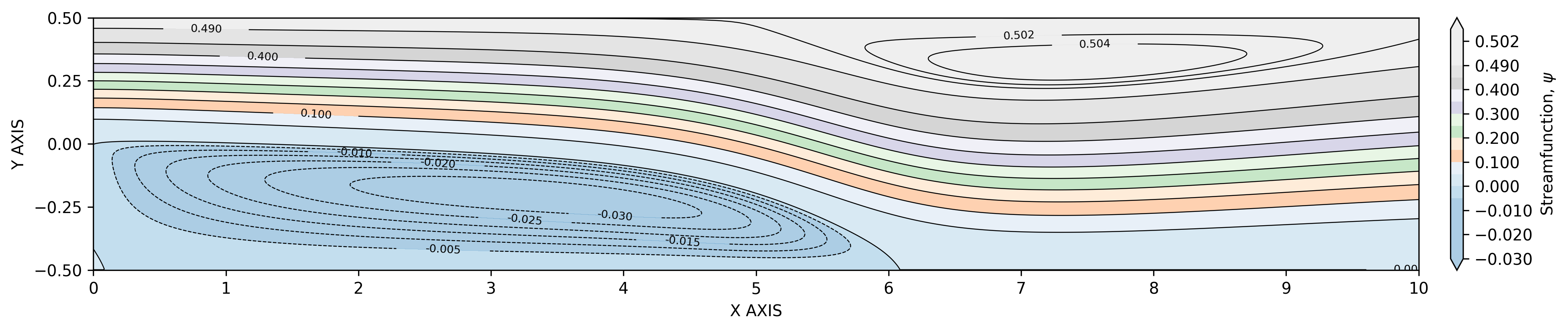
Fig. 14 Streamfunction contours at steady state.

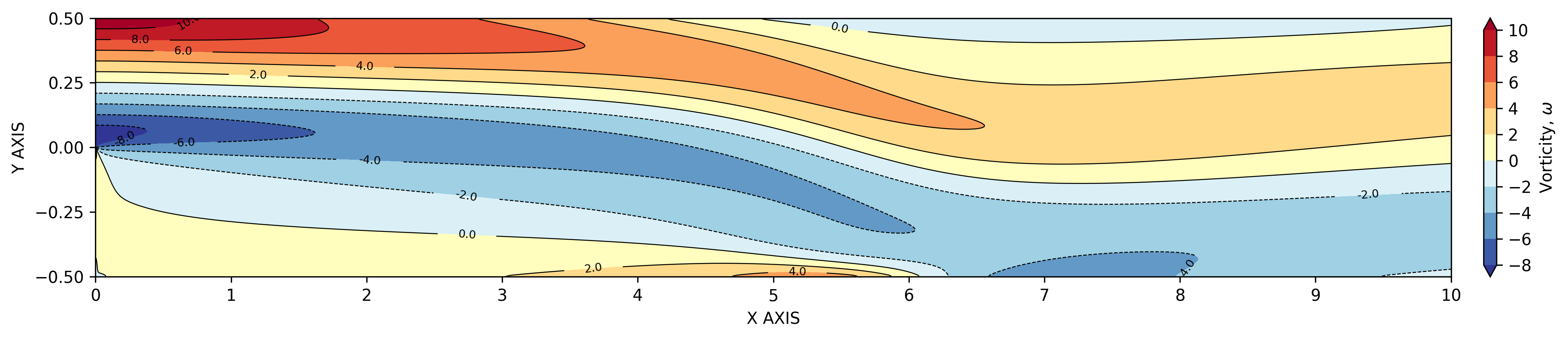
Fig. 15 Vorticity contours at steady state.

The horizontal velocity profiles at \(x=7\) and \(x=15\) can be used to compare the MFIX-Exa solution with Gartling’s tabulated results [Gar90]. The figure below includes several uniformly refined meshes, labeled by the number of cells in the \(x\) and \(y\) directions.

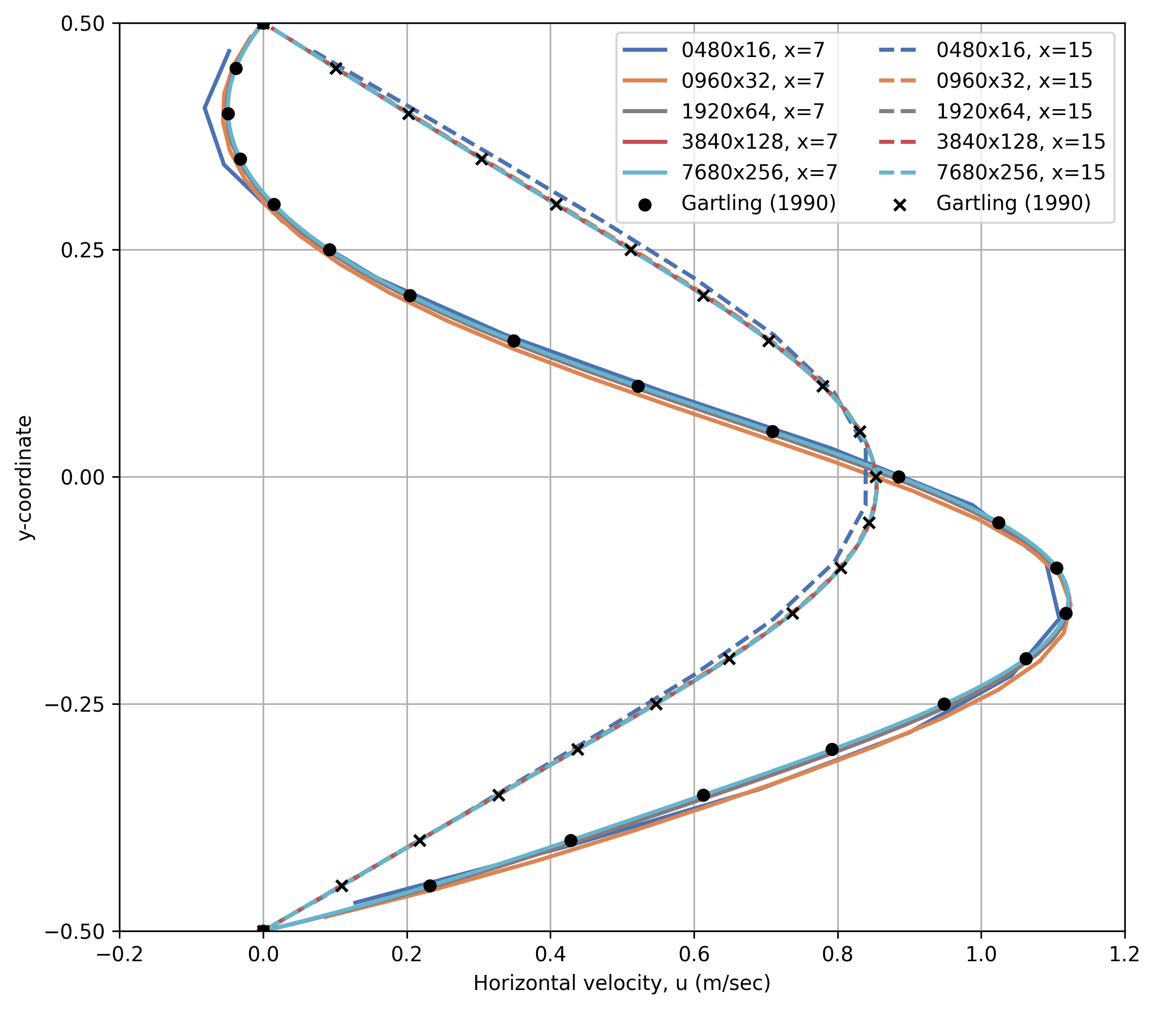
Fig. 16 Horizontal velocity profiles compared with Gartling [Gar90].

The horizontal velocity is well predicted even on the coarsest mesh: all five grids agree closely with Gartling’s data [Gar90] at both \(x=7\) and \(x=15\), with only modest, monotonically shrinking differences as the mesh is refined.

The vertical velocity tells a different story. At \(x=15\), downstream of reattachment, \(v\) is small in magnitude and every mesh – including the coarsest – agrees well with Gartling’s data [Gar90]. At \(x=7\), however, which sits inside the primary recirculation region, the two coarsest meshes (480x16 and 960x32) fail to capture the profile. The solution only becomes qualitatively correct at 1920x64.

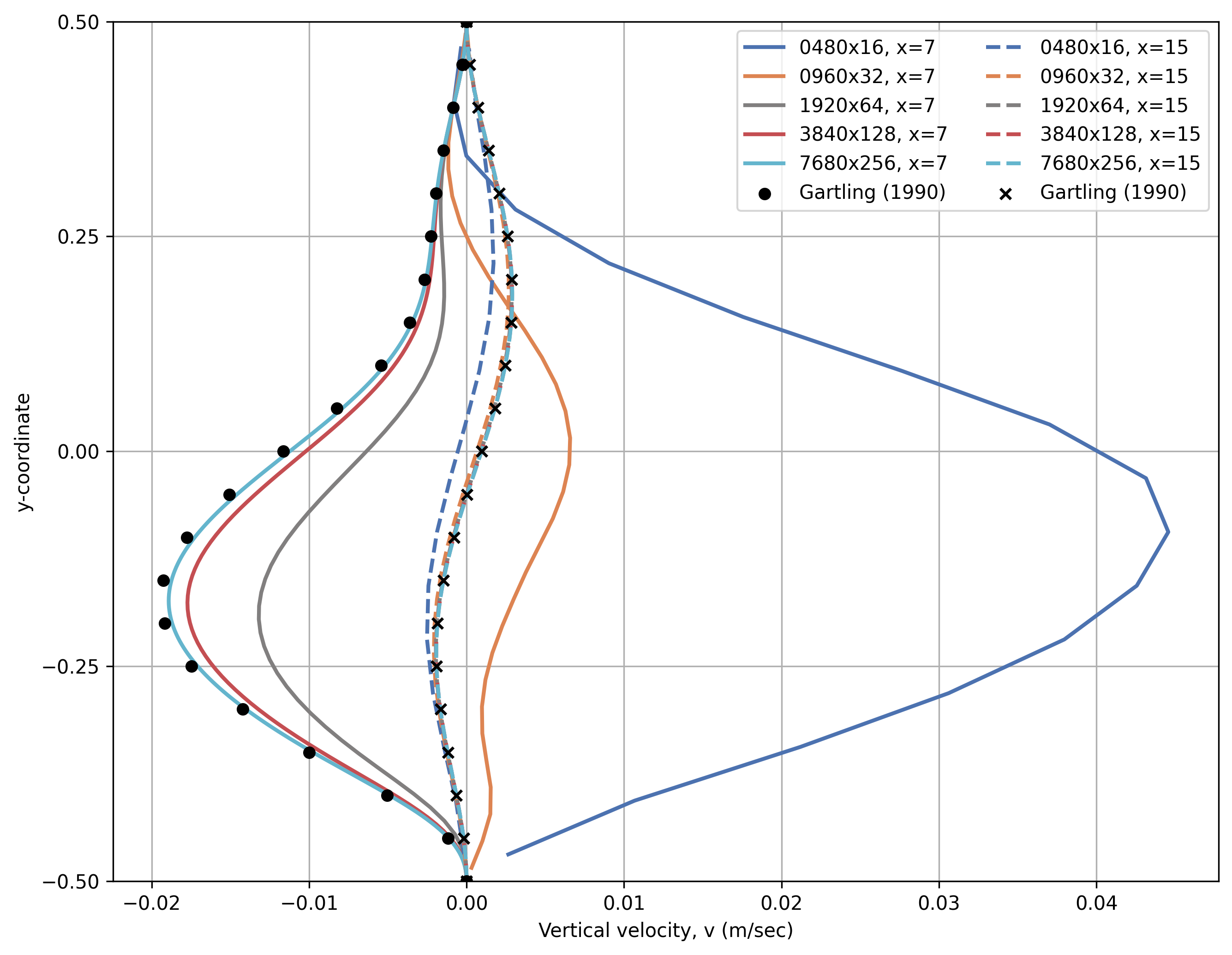
Fig. 17 Vertical velocity profiles compared with Gartling [Gar90].

This contrast is expected rather than concerning: \(u\) is the dominant, streamwise velocity component and is comparatively insensitive to resolution, while \(v\) at \(x=7\) is a small-magnitude, secondary quantity generated entirely by the curvature of the shear layer bounding the recirculation zone – the same near-wall region identified in Grid Convergence as needing the finest resolution to correctly locate the separation and reattachment points. A grid coarse enough to under-resolve that shear layer can still reproduce \(u\) reasonably well while getting \(v\) qualitatively wrong.

The pressure along the upper and lower walls is another useful comparison quantity. The plot below shows the pressure profiles from the finest mesh.

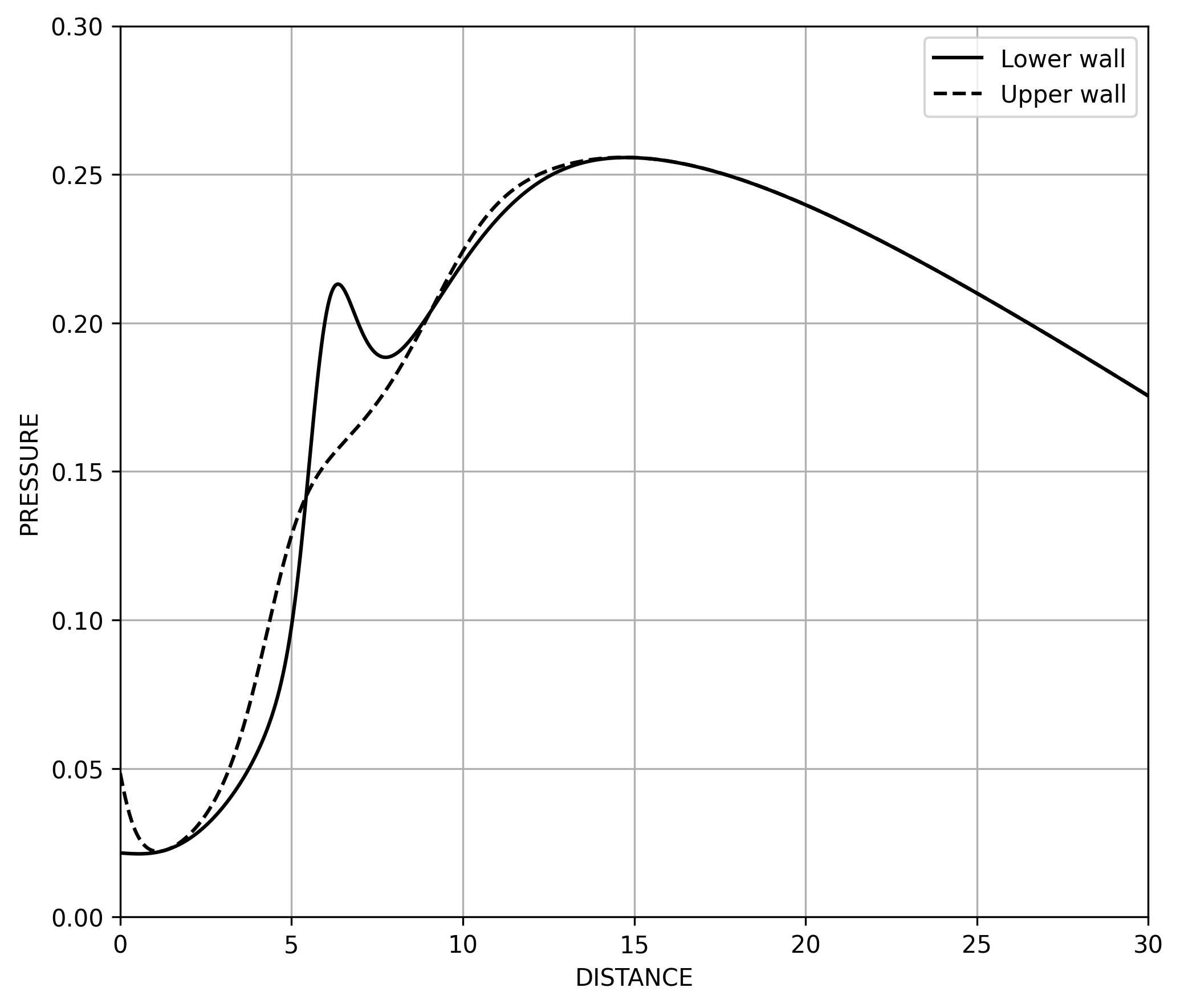
Fig. 18 Pressure profiles along the upper and lower channel walls.

Grid Convergence

To confirm that the reported comparisons are grid converged, the case was run on five uniformly refined meshes, labeled by the number of cells in the \(x\) and \(y\) directions (480x16, 960x32, 1920x64, 3840x128, and 7680x256). For each mesh, the lower- and upper-wall recirculation zones are characterized the same way Gartling [Gar90] does in Tables II and III:

• the vortex center is located as the extremum of the computed streamfunction within each recirculation zone,

• the streamfunction and vorticity are evaluated at that location, and

• the separation and reattachment points are located from the zero-crossings of the wall shear stress, \(\tau = \mu\, \partial u/\partial y\), using linear interpolation between grid points, following the same method Gartling describes.

Lower-wall eddy

Table 4 Lower-wall eddy vs. mesh resolution (cf. Gartling [Gar90], Table II)

Mesh	Vortex center \((x, y)\)	\(\psi\)	\(\omega\)	\(L_1\)
480x16	(2.9062, -0.2188)	-0.0299	-2.2402	4.9546
960x32	(3.2344, -0.2031)	-0.0331	-2.2513	5.8432
1920x64	(3.4453, -0.2109)	-0.0339	-2.2398	6.0420
3840x128	(3.4180, -0.2070)	-0.0341	-2.2488	6.0869
7680x256	(3.4043, -0.2051)	-0.0342	-2.2595	6.0951
Gartling (1990)	(3.35, -0.20)	-0.0342	-2.283	6.10

Richardson extrapolation on the reattachment length \(L_1\) gives an observed order of accuracy of \(p \approx 2.1\)-\(2.5\) across the three available triplets of meshes, consistent with the nominal second-order accuracy of the numerical scheme. Using the finest triplet (1920x64, 3840x128, 7680x256), \(p \approx 2.45\) and the extrapolated value is \(L_1(\Delta x \to 0) \approx 6.097\), matching Gartling’s [Gar90] reported value of 6.10 to within 0.05%.

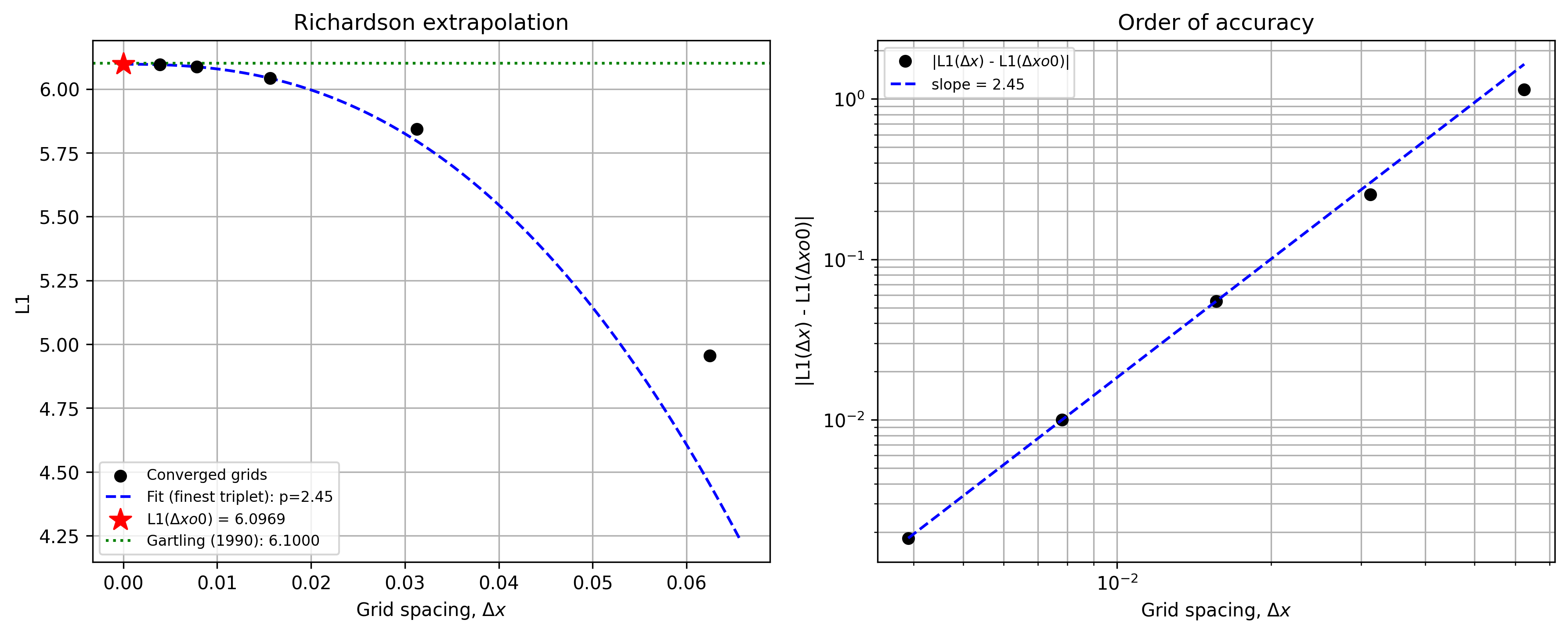
Fig. 19 Richardson extrapolation of the lower-wall reattachment length \(L_1\).

Upper-wall eddy

Table 5 Upper-wall eddy vs. mesh resolution (cf. Gartling [Gar90], Table III)

Mesh	Vortex center \((x, y)\)	\(\psi\)	\(\omega\)	Separation \((x, y)\)	Reattachment \((x, y)\)	\(L_u\)
480x16	(6.9688, 0.2812)	0.5105	1.6707	(3.4912, 0.50)	(9.7500, 0.50)	6.2588
960x32	(7.2969, 0.2969)	0.5072	1.3218	(4.4186, 0.50)	(10.5215, 0.50)	6.1029
1920x64	(7.4609, 0.3203)	0.5067	1.0892	(4.7017, 0.50)	(10.5332, 0.50)	5.8315
3840x128	(7.4492, 0.3164)	0.5066	1.1344	(4.7939, 0.50)	(10.5113, 0.50)	5.7174
7680x256	(7.4473, 0.3145)	0.5065	1.1584	(4.8268, 0.50)	(10.4965, 0.50)	5.6697
Gartling (1990)	(7.40, 0.30)	0.5064	1.322	(4.85, 0.50)	(10.48, 0.50)	5.63

Richardson extrapolation on the upper-wall recirculation length \(L_u\) is more sensitive to mesh resolution than \(L_1\): the coarsest triplet (480x16, 960x32, 1920x64) gives an unphysical negative order of accuracy, which is not unexpected since the upper-wall separation point is a gradual, adverse-pressure-gradient-driven separation rather than the fixed, geometric separation at the step corner, and is correspondingly harder to resolve on coarse meshes. The two finer triplets are consistent with one another, \(p \approx 1.25\)-\(1.26\), giving an extrapolated value of \(L_u(\Delta x \to 0) \approx 5.635\), matching Gartling’s [Gar90] reported value of 5.63 to within 0.1%.

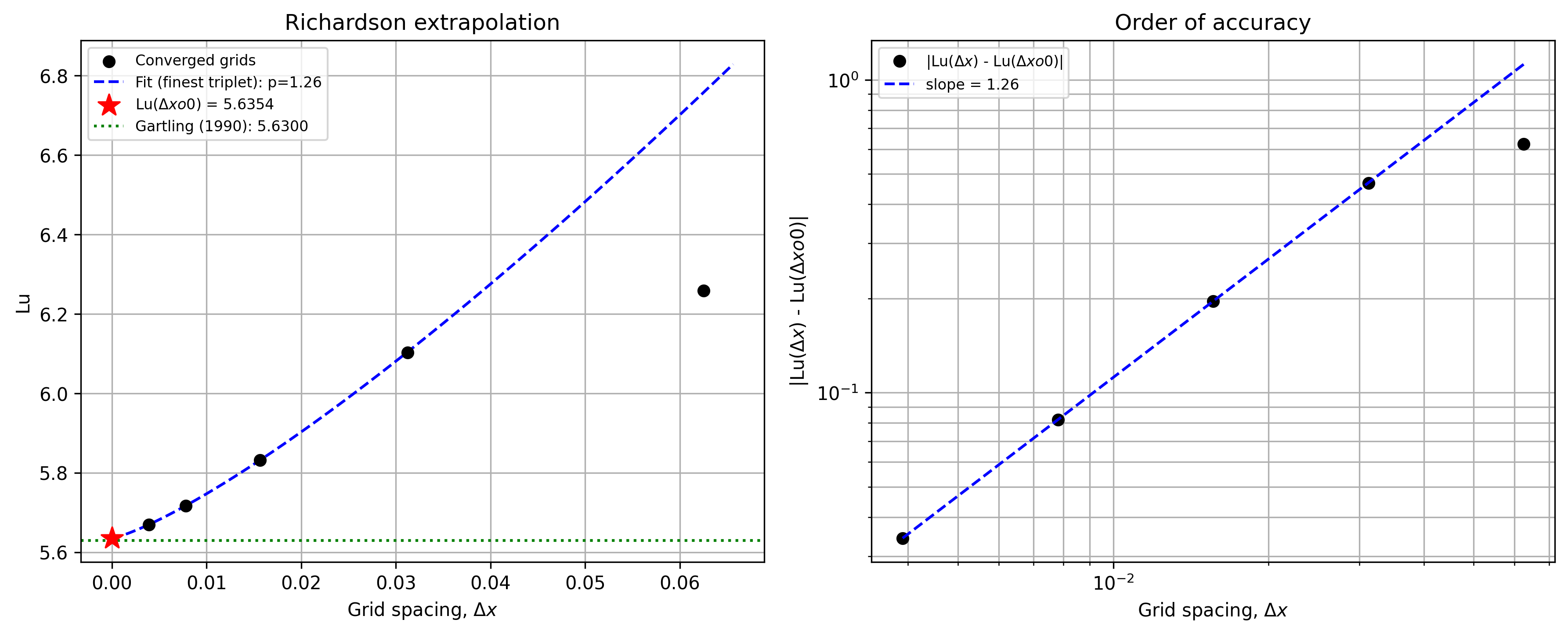
Fig. 20 Richardson extrapolation of the upper-wall recirculation length \(L_u\).

Taken together, the vortex-center locations and strengths agree with Gartling’s finest-mesh results [Gar90] to within 1-2% even at moderate resolution, and the Richardson-extrapolated separation/reattachment lengths for both recirculation zones agree with his reported values to within 0.1%.