Unsteady flow around a sphere

This tutorial extends the steady flow around a sphere case to \(Re=300\), where the wake sheds periodically as a chain of hairpin vortices rather than settling into a fixed recirculation bubble. The geometry, domain, and mesh are unchanged from the steady case; only the Reynolds number and the time-advance scheme differ. The drag coefficient and vortex-shedding frequency are computed as part of the analysis.

Features

• Incompressible fluid flow.

• Unsteady (transient) time advance using the Godunov scheme.

• The same fully three-dimensional embedded-boundary sphere geometry as the steady tutorial.

• A transient, space-and-time-dependent inflow velocity used to seed the wake instability.

• Surface-force (drag and side-force) reporting on the embedded boundary.

• Statistical (batch-means) analysis of the drag coefficient and Strouhal number, with comparison against Johnson & Patel (1999) [JP99].

Case description

The sphere, domain, and mesh are identical to the steady tutorial: diameter \(D=1\), centered at the origin, with the domain extending 8 diameters upstream, 16 diameters downstream, and 8 diameters radially in \(y\) and \(z\), resolved at 16 cells/diameter (384x256x256).

The Reynolds number is raised to

\[Re = \frac{\rho\, U_\infty\, D}{\mu} = 300, \qquad \mu = 0.0033333,\]

with \(\rho=1\) and \(U_\infty=1\) unchanged. At this Reynolds number the wake sheds periodically as a chain of hairpin vortices with planar (not axisymmetric) symmetry (Sakamoto & Haniu [SH90]); the transition from the steady axisymmetric wake used in the \(Re=100\) tutorial passes through an intermediate steady-but-non-axisymmetric regime around \(Re\approx210\)-\(270\) before periodic shedding begins around \(Re\approx270\)-\(300\).

Seeding the instability

The steady axisymmetric solution remains a mathematically valid, though unstable, equilibrium at \(Re=300\). A solver that preserves the problem’s symmetry exactly can sit near that equilibrium indefinitely without something to break the symmetry. Rather than rely on numerical noise to trigger the transition, the inflow velocity is given a small, transient, spatially localized perturbation, antisymmetric in \(y\), that decays away after roughly the first ten time units:

bc.inflow.fluid.velocity = "1.0 + 0.05*exp(-t/2.0)*y*exp(-(y*y+z*z))"

This has the side effect of fixing the shedding plane to the \(x\)- \(y\) plane, rather than leaving the orientation to arbitrary numerical noise – a deliberate choice for a reproducible tutorial result. The \(z\)-force on the sphere stays at floating-point roundoff throughout the run, confirming the wake organizes into the intended plane.

Important input sections

The fluid viscosity sets the Reynolds number:

fluid.viscosity.molecular.model = constant
fluid.viscosity.molecular.constant = 0.0033333

Genuine unsteady time advance is used in place of the steady tutorial’s pseudo steady-state iteration, with the Godunov advection scheme and a raised CFL number:

mfix.advection_type = Godunov
mfix.cfl = 0.9

mfix.dt_min = 1.0e-6
mfix.dt_max = 0.1

mfix.stop_time = 1000.0

Explicit, CFL-limited unsteady time advance is more sensitive to severely cut EB cells than the steady tutorial’s pseudo-time advance was – a very small cut cell can otherwise force either an unphysically small timestep or outright instability. State redistribution addresses this by redistributing the update from small cut cells into their larger neighbors:

mfix.redistribution_type = StateRedist
mfix.correction_small_volfrac = 1.e-4

The eb_drag report is sampled far more frequently than in the steady tutorial, to adequately resolve the shedding frequency:

mfix.reports.eb_drag.regions = eb_sphere
mfix.reports.eb_drag.eb_sphere.int = 3

Note

The complete input file is located in the MFIX-Exa source directory as tutorials/fluid/inputs.unsteady-flow-around-sphere

Post-processing

The eb_drag report gives the drag coefficient \(C_d\) and the lateral force coefficients \(C_y\), \(C_z\) over the full run:

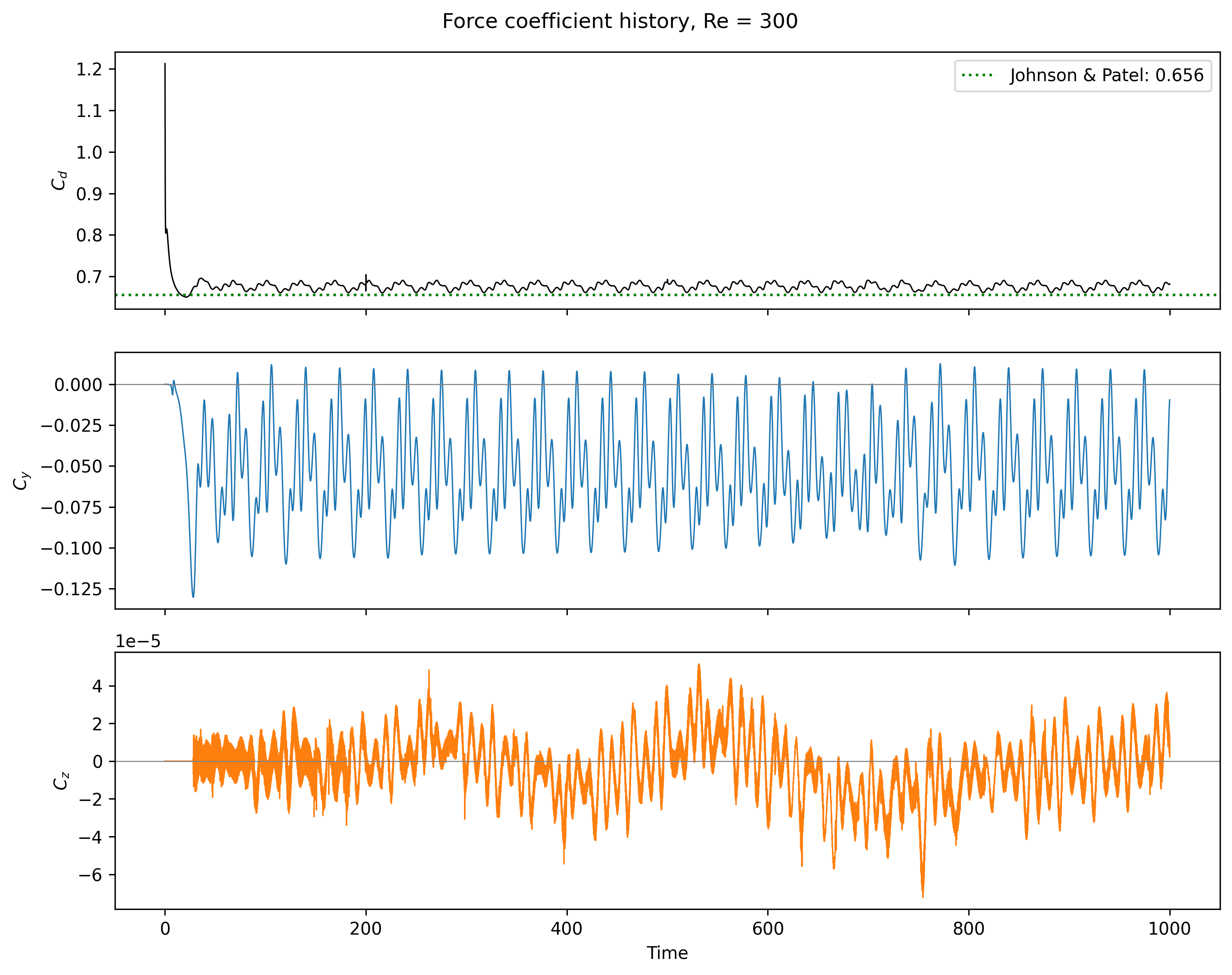
Fig. 22 Force coefficient history, \(Re=300\).

\(C_z\) sits at floating-point roundoff throughout, confirming the wake sheds in the intended plane. \(C_y\) carries a persistent negative mean rather than oscillating about zero – consistent with the “planar” wake character described in the literature for this Reynolds-number range, where the wake settles into a steady deflection with periodic shedding superimposed, rather than a simple side-to-side oscillation.

A windowed mean/standard-deviation view of \(C_y\) shows a slow amplitude modulation, with a period of roughly 34 time units, superimposed on the underlying shedding oscillation:

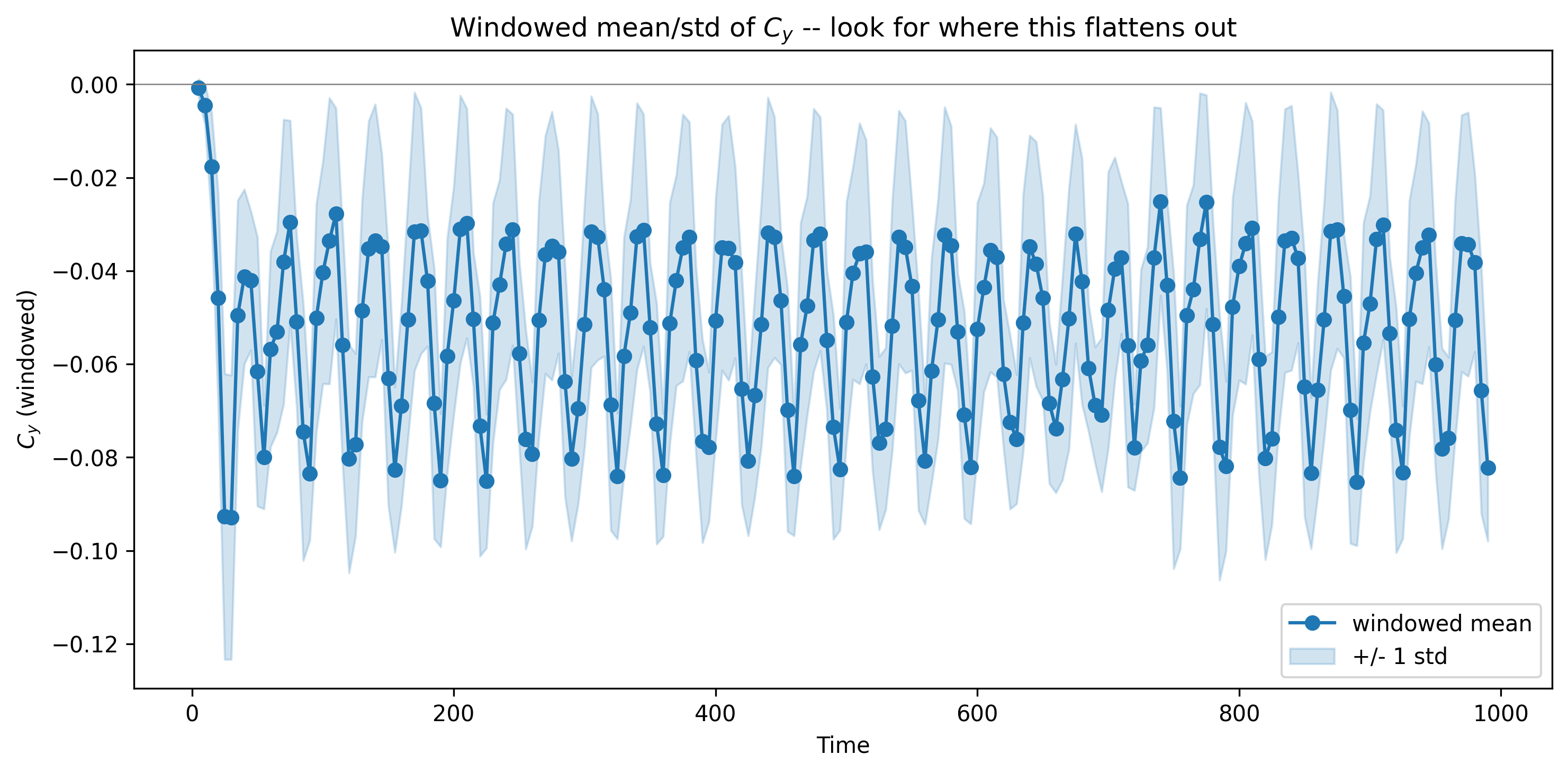
Fig. 23 Windowed mean and standard deviation of \(C_y\).

This modulation does not decay over the roughly 970 time units recorded after the initial transient, indicating it is a persistent secondary feature of the flow at this resolution rather than an artifact of insufficient run time. It is directly visible in the frequency spectrum of \(C_y\) as sidebands evenly spaced around the true shedding frequency by the modulation frequency – amplitude modulation of a single carrier, not several independent shedding modes:

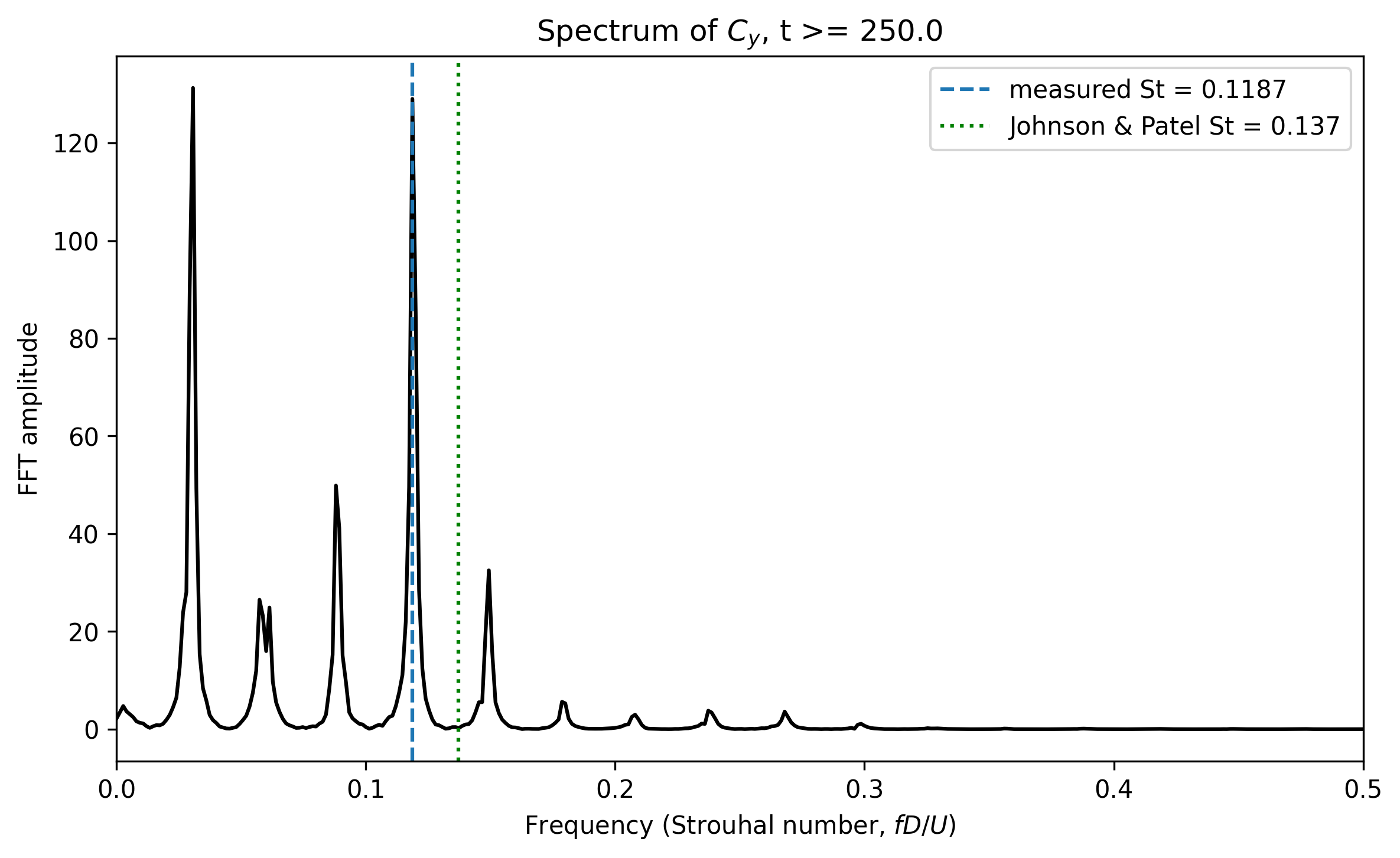
Fig. 24 Spectrum of \(C_y\), settled window.

Statistical analysis

The drag coefficient and shedding (Strouhal) frequency were each estimated using the batch-means method: the settled portion of the record (\(t\ge250\)) was split into seven non-overlapping 100-time-unit windows, each window’s quantity was estimated independently, and a t-distribution interval was computed on the resulting sample. Because these windows are consecutive segments of one continuous run rather than independent repeated experiments, this interval should be read as the spread of the estimate within this run, not a formal confidence interval over repeated realizations.

Table 8 Batch-means results vs. Johnson & Patel (1999), \(Re=300\)

Quantity	Mean	95% interval	Reference	% difference
\(C_d\)	0.6765	(0.6760, 0.6770)	0.656	+3.1%
\(St\)	0.1191	(0.1186, 0.1195)	0.137	-13.1%

Both intervals are narrow enough that the reference value falls clearly outside each one – these are small but real, well-resolved discrepancies rather than run-to-run noise. The drag coefficient is close to the reference; the shedding frequency is not. No dedicated grid-refinement study was performed for this unsteady case (unlike the steady tutorial), so mesh resolution is a plausible, though unconfirmed, contributor to both gaps.

Flow visualization

A single mid-plane slice, colored by out-of-plane vorticity, shows the meandering wake:

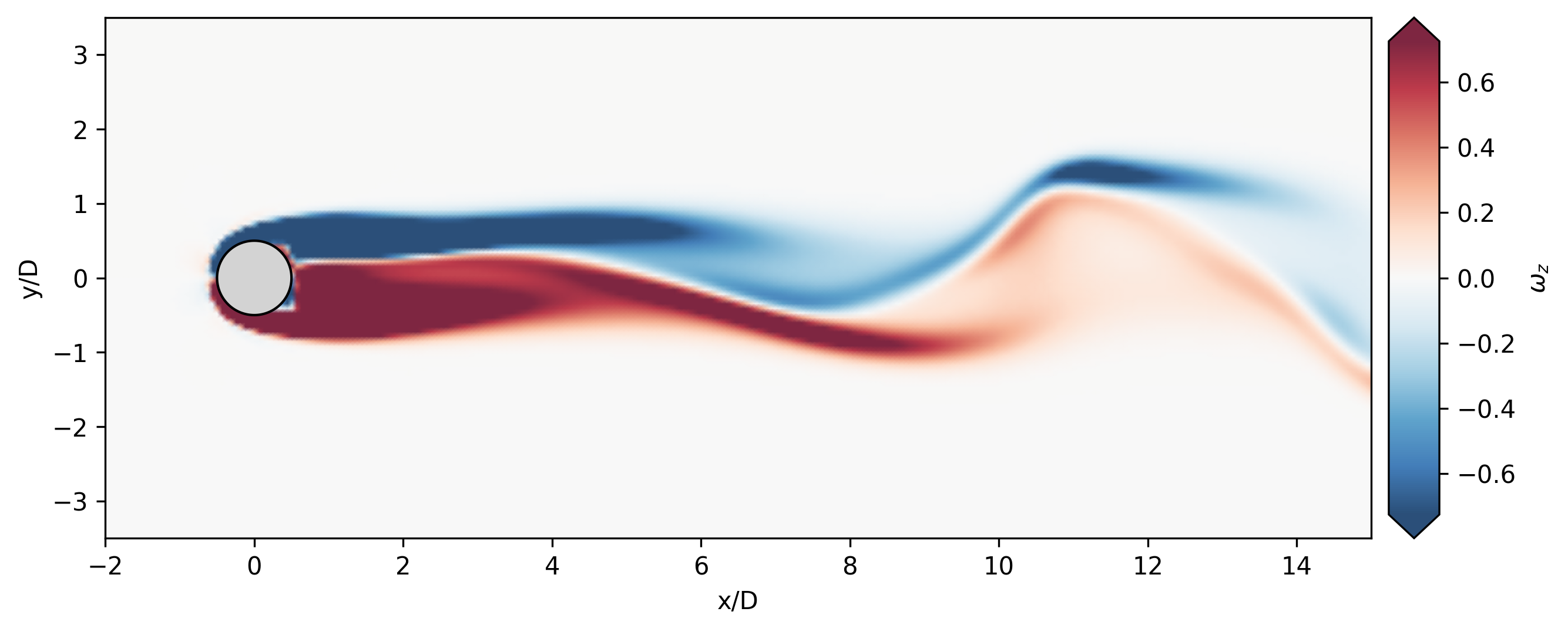
Fig. 25 Out-of-plane vorticity, mid-plane slice, \(Re=300\).

A 2D slice cannot show the shedding process itself, since the shed structures are inherently three-dimensional. An animation of Q-criterion isosurfaces, colored by velocity magnitude and generated in ParaView, shows the wake organizing into a pair of counter-rotating streamwise vortex legs that periodically pinch off into discrete hairpin loops and convect downstream.