Steady natural convection in a differentially heated cavity

This tutorial sets up buoyancy-driven flow in a closed, differentially heated square cavity – the classical de Vahl Davis benchmark [dVD83]. Unlike the earlier sphere tutorials, this case exercises MFIX-Exa’s energy equation and ideal-gas equation of state: buoyancy comes directly from a real density variation with temperature, not a linearized Boussinesq source term (MFIX-Exa has no Boussinesq mode). A grid-refinement study validates the computed Nusselt number against the benchmark.

Features

• Buoyancy-driven fluid flow.

• Ideal-gas equation of state in a sealed (closed) domain – mfix.constraint = IdealGasClosedSystem.

• Steady-state pseudo-time advance.

• Vertical hot/cold walls represented as an embedded boundary; adiabatic top/bottom walls handled as plain domain boundary conditions.

• Quasi-2D domain using a thin, periodic spanwise (\(z\)) direction.

• Grid-refinement study (\(64^2\), \(128^2\), \(256^2\)) with Richardson extrapolation of the wall Nusselt number, compared against de Vahl Davis [dVD83] and Hortmann et al. [HPericS90].

Case description

The cavity is a unit cube in \(x\)-\(y\) with characteristic length \(L=1\text{ m}\), thin and periodic in \(z\). The left (\(x=-0.5\)) and right (\(x=+0.5\)) walls are held at fixed temperatures \(T_h=310\text{ K}\) and \(T_l=290\text{ K}\). The top and bottom walls are adiabatic and no-slip. Gravity points in the \(-y\) direction. This case is characterized by the Rayleigh number (\(Ra\)) and Prandtl number (\(Pr\)):

\[Ra = \frac{g\,\beta\,\Delta T\,L^3}{\nu\,\alpha} = 1\times10^6, \qquad Pr = \frac{\mu c_p}{\kappa} = 0.717\]

where \(\beta=1/T_{ref}\) for an ideal gas fluid.

This setup is a near-Boussinesq validation case; therefore, the temperature difference is kept small relative to the reference temperature \(T_{ref} = 300\text{ K}\):

\[\frac{\Delta T}{T_{ref}} = \frac{20}{300} = 6.7\%\]

This approach keeps the ideal-gas solve close to the Boussinesq limit that the classical benchmark assumes. (A companion case at \(\Delta T/T_{ref}=120\%\), validating against the compressible benchmark of Le Quéré [LQWP+05] instead, is a natural extension – see below.)

The viscosity (\(\mu\)) and thermal conductivity (\(\kappa\)) are solved for from the target \(Ra\), \(Pr\), \(\Delta T\), and \(L\).

\[\mu = 8.061\times10^{-4}\text{ Pa}\cdot\text{s}, \qquad \kappa = 1.1292\text{ W/(m}\cdot\text{K)}\]

The specific heat and molecular weight are prescribed constants, \(C_p=1004.5\text{ J/(kg}\cdot\text{K)}\) and \(M=0.028970\text{ kg/mol}\), respectively. The values are checked for a physically valid ideal gas before use:

\[C_v = C_p - \frac{R}{M} = 1004.5 - \frac{8.31446}{0.028970} = 717.5\text{ J/(kg}\cdot\text{K)} > 0, \qquad \gamma = C_p/C_v \approx 1.400\]

Warning

When choosing fluid properties to satisfy specific dimensionless groups (like \(Ra\) and \(Pr\)), always verify that the resulting thermodynamic properties remain physical. Arbitrarily adjusting \(C_p\) or molecular weight without this check can accidentally yield a negative constant-volume specific heat (\(C_v \le 0\)), leading to an unphysical ideal gas state and solver divergence.

Important input sections

The domain is a unit cube, periodic in \(z\):

geometry.is_periodic  =  0       0       1
geometry.prob_lo      = -0.5  -0.5   0.0
geometry.prob_hi      =  0.5   0.5   0.125

amr.n_cell = 64  64  8

The hot/cold walls are represented as an embedded boundary covering the \(x\) faces of the domain; \(y\) (top/bottom) are defined as no-slip walls and handled by ordinary domain boundary conditions, and \(z\) is periodic:

mfix.geometry = box

box.Lo = -0.5  -1.0  -1.0
box.Hi =  0.5   1.0   1.0

box.internal_flow = true
box.offset        = 1.e-8

...

bc.left                          =  eb
bc.left.eb.normal                =  1. 0. 0.
bc.left.eb.temperature           =  constant
bc.left.eb.temperature.constant  =  310.          # Th

bc.right                          =  eb
bc.right.eb.normal                = -1. 0. 0.
bc.right.eb.temperature           =  constant
bc.right.eb.temperature.constant  =  290.          # Tl

bc.top    = no-slip     # adiabatic (no temperature spec)
bc.bottom = no-slip

The energy equation and the ideal-gas equation of state are enabled together in a sealed domain:

mfix.advect_density  = 1
mfix.advect_enthalpy = 1
mfix.constraint      = IdealGasClosedSystem

The calculated viscosity (\(\mu\)), thermal conductivity (\(\kappa\)), and prescribed specific heat ((\(C_p\))) are set as constant fluid properties in the configuration deck:

fluid.specific_heat.model           = constant
fluid.specific_heat.constant        = 1004.5

fluid.viscosity.molecular.model     = constant
fluid.viscosity.molecular.constant  = 8.061e-4

fluid.thermal_conductivity.model    = constant
fluid.thermal_conductivity.constant = 1.1292

The case runs to a pseudo steady state:

mfix.steady_state         = 1
mfix.steady_state_tol     = 1.e-6
mfix.steady_state_maxiter = 100000

mfix.dt_max = 1.0e-2

Note

The complete input file is located in the MFIX-Exa source directory as tutorials/fluid/inputs.steady-natural-convection-cavity

Post-processing

Nusselt number

The local Nusselt number at each vertical wall is

\[Nu = \frac{L}{T_h-T_l}\left.\frac{\partial T}{\partial x}\right|_{wall}\]

computed with a second-order, one-sided finite-difference stencil on the first three cell-center planes off the wall and averaged over \(y\). At the left (hot) wall, this is evaluated as:

\[\left.\frac{\partial T}{\partial x}\right|_{wall} = \frac{-2T_1+3T_2-T_3}{\Delta x}\]

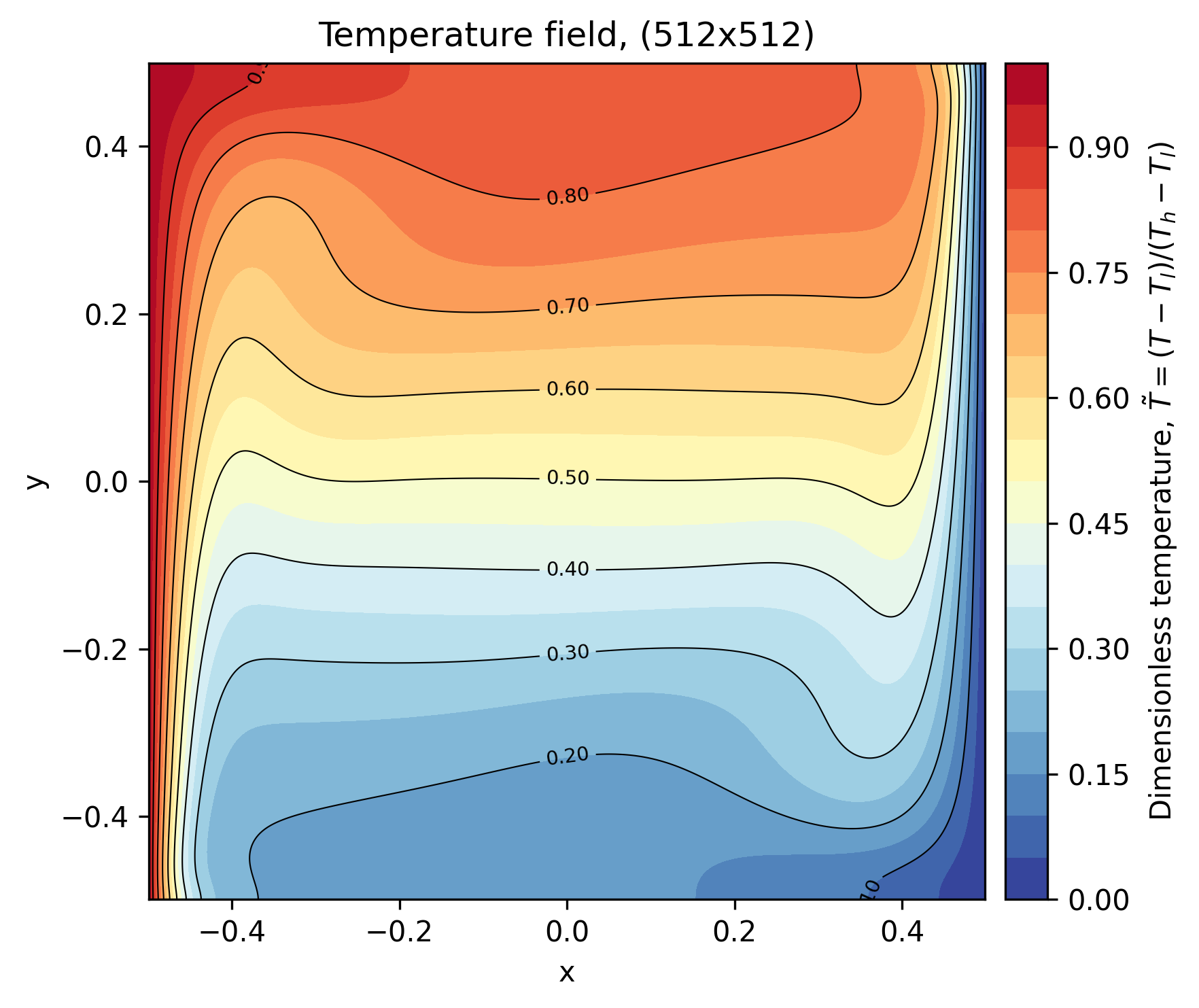
Fig. 26 Dimensionless temperature field \(\tilde{T}=(T-T_l)/(T_h-T_l)\), \(128^2\) grid.

The field shows the expected structure for \(Ra=10^6\): thin thermal boundary layers along the hot and cold walls, a stably stratified core, and a single large recirculating cell—consistent with de Vahl Davis’s description at this Rayleigh number.

Grid convergence

Table 9 Wall Nusselt number vs. grid, Ra=1e6 :header-rows: 1

Mesh	\(Nu_{xmin}\) (hot wall)	\(Nu_{xmax}\) (cold wall)
\(64\times64\)	9.7986	9.8098
\(128\times128\)	9.0170	9.0240
\(256\times256\)	8.8572	8.8584
\(512\times512\)	8.8331	8.8331
de Vahl Davis / Hortmann et al.	8.80 - 8.83	8.80 - 8.83

Richardson extrapolation across the three finest grids gives an observed order of accuracy of \(p\approx2.74\) (hot wall) / \(2.72\) (cold wall). The extrapolated value at the continuum limit (\(\Delta x\to0\)) lands at the benchmark values from de Vahl Davis [dVD83] and Hortmann et al. [HPericS90]:

Table 10 Richardson extrapolation vs. benchmark literature :header-rows: 1

Quantity	Observed order \(p\)	Extrapolated (\(\Delta x\to0\))	Reference
\(Nu_{xmin}\)	2.741	8.8289	8.82
\(Nu_{xmax}\)	2.717	8.8287	8.82

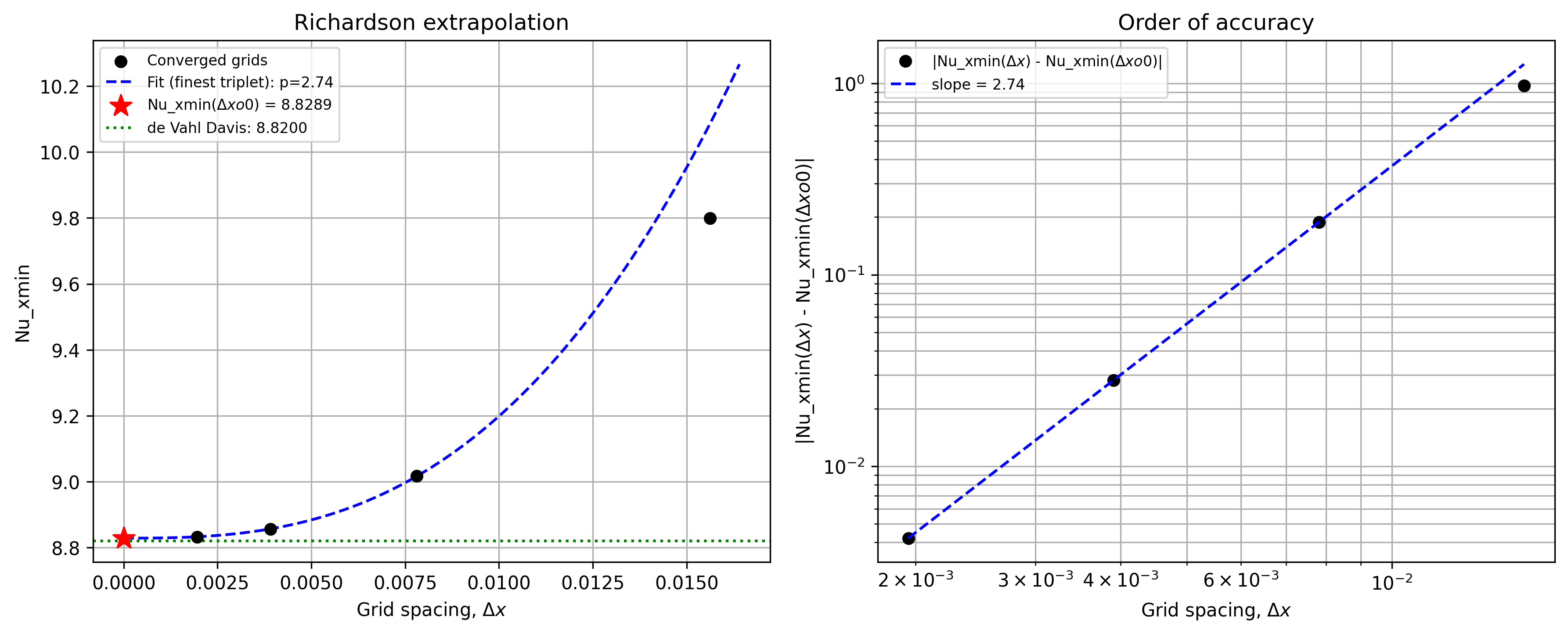
Fig. 27 Richardson extrapolation, \(Nu_{xmin}\) (hot wall).

Both walls agree with each other in \(Nu\) at every grid level, as expected from overall energy balance at steady state, and both converge cleanly toward the classical benchmark as the mesh is refined.

Steady-state convergence check

mfix.steady_state_tol being satisfied confirms the residual dropped below tolerance, not that the converged state is the physically correct one Tracking \(Nu\) and the mean thermodynamic pressure over the last several plotfiles confirms a genuine plateau rather than a false-positive stop:

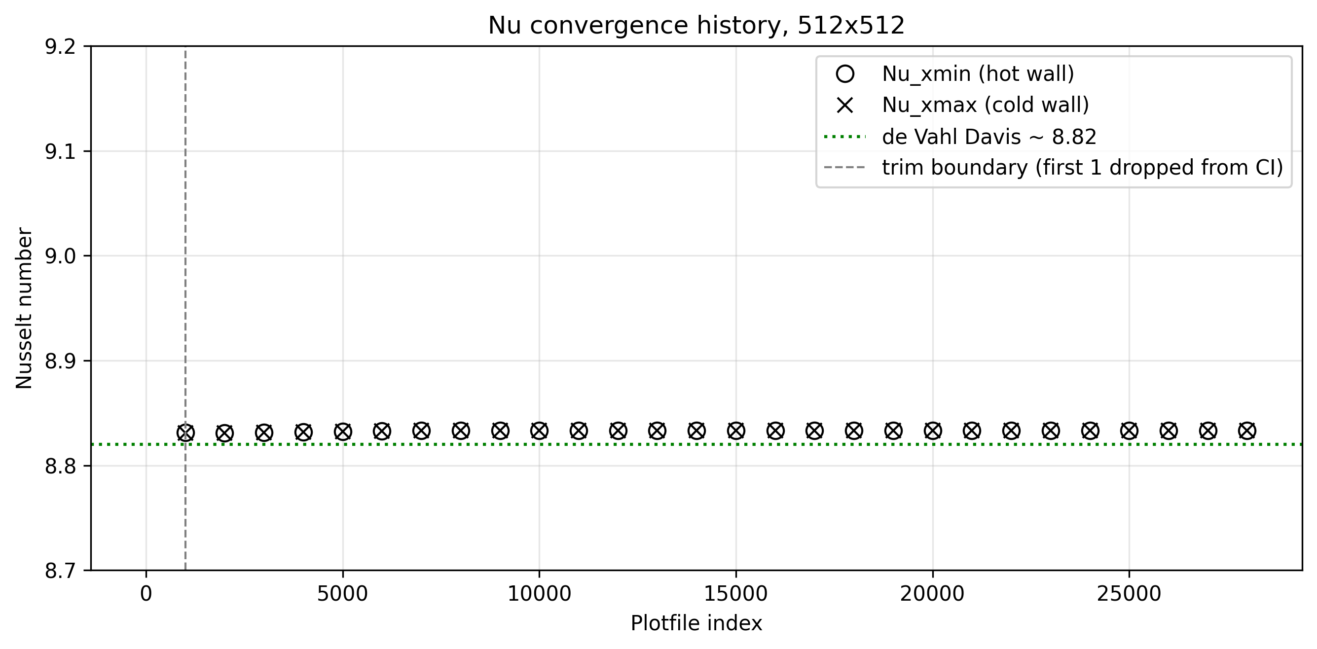
Fig. 28 \(Nu\) convergence history, \(512\times512\) grid.

Excluding the initial transient (first output only), a block-bootstrap estimate over the last 28 plotfiles gives \(Nu_{xmin}=8.83289\pm0.00032\) and \(Nu_{xmax}=8.83290\pm0.00035\) (95% CI)—a tight, flat plateau consistent with the point value used in the grid-convergence table above, not a still-drifting solution.

Thermodynamic pressure check

As a second, independent and mesh-cheap validation check, mass conservation in the closed ideal-gas domain fixes the domain-mean thermodynamic pressure relative to the wall temperatures. For a purely conductive profile, the pressure ratio evaluates to the ratio of the logarithmic mean wall temperature to the reference temperature:

\[\frac{P_{mean}}{P_o} = \frac{T_{lm}}{T_{ref}}, \qquad T_{lm} = \frac{T_h-T_l}{\ln(T_h/T_l)}\]

where \(P_o\) is the initial operating pressure of the closed system.

For this case, \(T_{lm}/T_{ref}=0.99963\), matching the computed \(P_{mean}/P_o=0.99960\) to within 0.004%—and essentially unchanged across all grids (0.999592 / 0.999599 / 0.999600 / 0.999600). Since this is a domain-integral quantity dominated by the fixed wall temperatures rather than a locally resolved wall gradient, it serves as a highly effective, computationally cheap sanity check that is already converged on the coarsest mesh, well before \(Nu\) itself finishes converging.

Extensions

• A companion case at \(\Delta T/T_{ref}=120\%\) (\(T_h=960\text{ K}\), \(T_l=240\text{ K}\), \(T_{ref}=600\text{ K}\), same \(Ra\), \(Pr\)) tests how far the ideal-gas solve departs from the Boussinesq benchmark as the temperature difference grows, validated instead against Le Quere [LQWP+05]. The thermodynamic-pressure check above is expected to show a much larger, and more convection-sensitive, departure from its pure-conduction prediction at that \(\Delta T\).

• Radiative coupling between the walls (not covered here) is a further extension of the pure-convection case [LBGandjalikhanNassab+11].