Steady flow around a sphere

This tutorial sets up steady, incompressible flow past an isolated sphere at \(Re=100\), well within the regime where the wake is steady and axisymmetric. It is the first tutorial in this series to use a fully three-dimensional embedded-boundary geometry – both the steady flow past a cylinder and backward-facing step tutorials are effectively two-dimensional, using a periodic or resolved-but-extruded spanwise direction. The sphere drag coefficient and wake recirculation length are computed as part of the analysis.

Features

• Incompressible fluid flow.

• Steady-state pseudo-time advance.

• Fully three-dimensional embedded-boundary sphere geometry.

• Uniform freestream mass inflow, pressure outlet, and free-slip lateral boundaries approximating an unconfined far field.

• Plotfile output for velocity and pressure.

• Surface-force (drag) reporting on the embedded boundary.

• Comparison against the Schiller-Naumann drag correlation and the Johnson & Patel (1999) [JP99] / Taneda (1956) [Tan56] recirculation-length data.

• A four-level grid-refinement study.

Case description

The sphere has diameter \(D=1\) (radius \(r=0.5\)) and is centered at the origin. The domain extends 8 diameters upstream, 16 diameters downstream, and 8 diameters radially in \(y\) and \(z\):

\[-8 \le x \le 16, \qquad -8 \le y \le 8, \qquad -8 \le z \le 8,\]

giving a blockage ratio (frontal sphere area to domain cross-section) of about 0.3%, small enough that the lateral boundaries have a negligible effect on the resolved flow.

The tutorial uses

\[\rho = 1,\qquad U_\infty = 1,\qquad D = 1,\qquad \mu = 0.01,\]

giving

\[Re = \frac{\rho\, U_\infty\, D}{\mu} = 100.\]

At this Reynolds number the wake is steady and axisymmetric about the flow direction; the transition to a steady but non-axisymmetric wake does not occur until \(Re \approx 212\), and vortex shedding does not begin until \(Re \approx 270\)-\(300\).

Important input sections

The sphere is defined through MFIX-Exa’s built-in sphere embedded-boundary geometry:

mfix.geometry = "sphere"

sphere.radius = 0.5
sphere.center = 0.0  0.0  0.0
sphere.internal_flow = false

Unlike the channel-flow cases in this series, the domain here represents an unconfined free stream rather than a physical enclosure, so the lateral boundaries use a free-slip condition instead of no-slip walls. The low- \(x\) face is a uniform mass inflow, and the high-\(x\) face is a pressure outlet:

bc.regions = inflow outflow side_ylo side_yhi side_zlo side_zhi

bc.inflow = mi
bc.inflow.fluid.density = 1.0
bc.inflow.fluid.inflow_type = velocity
bc.inflow.fluid.velocity = 1.0

bc.outflow = po
bc.outflow.pressure = 0.0

bc.side_ylo = slip
bc.side_yhi = slip
bc.side_zlo = slip
bc.side_zhi = slip

No boundary condition entry is needed for the sphere itself – embedded boundaries are no-slip by default. A separate region, slightly larger than the sphere, is used only to define where the drag report integrates:

regions.eb_sphere.shape = sphere
regions.eb_sphere.sphere.radius = 0.75
regions.eb_sphere.sphere.center = 0.0  0.0  0.0

mfix.reports.eb_drag.regions = eb_sphere
mfix.reports.eb_drag.eb_sphere.int = 500

The fluid viscosity sets the Reynolds number:

fluid.viscosity.molecular.model = constant
fluid.viscosity.molecular.constant = 0.01

As with the backward-facing-step case, the run uses the pseudo steady-state time advance:

mfix.steady_state = 1

mfix.steady_state_tol = 1.0e-6
mfix.steady_state_maxiter = 100000

Note

The complete input file is located in the MFIX-Exa source directory as tutorials/fluid/inputs.steady-flow-around-sphere

Post-processing

The run writes an AMReX plotfile named plt* every 5000 iterations into a directory, io, in the run directory. Each plotfile saves the fluid velocity field, vel_g, pressure, p_g, and volume fraction, volfrac. The eb_drag report writes a time history of the surface force on the sphere, from which the drag coefficient

\[C_d = \frac{F_x}{\tfrac{1}{2}\rho U_\infty^2 A}, \qquad A = \pi r^2,\]

is computed. All results were analyzed using a Jupyter notebook.

A mid-plane slice through the wake, with the in-plane velocity streamlines overlaid, shows the expected steady, axisymmetric single recirculation bubble immediately behind the sphere:

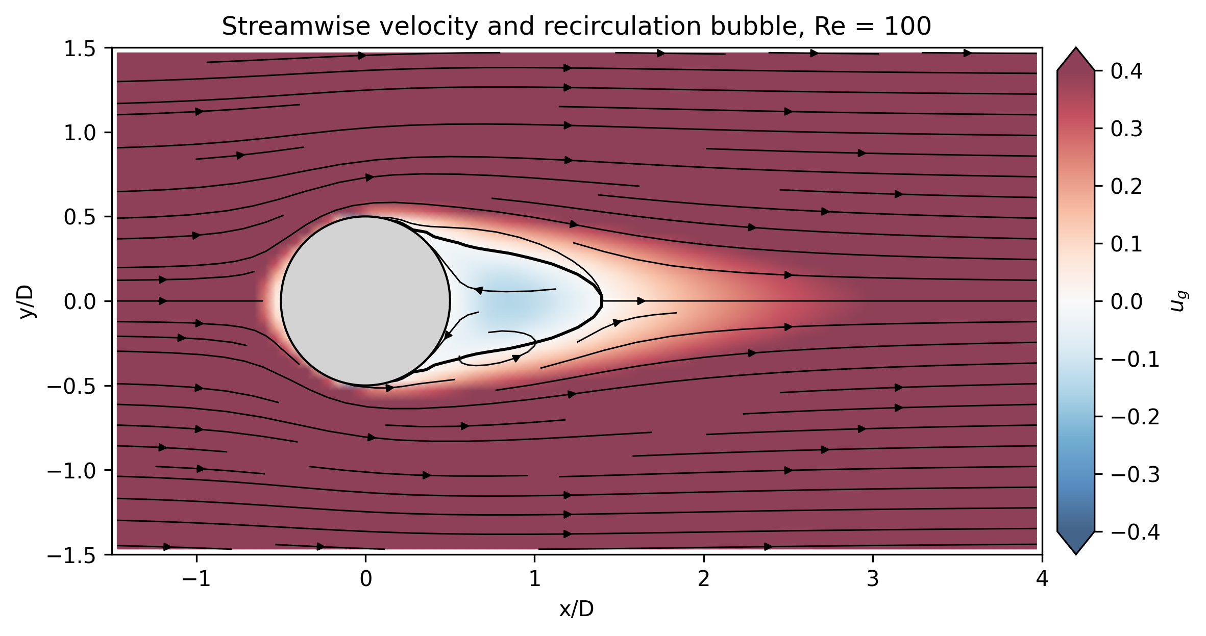
Fig. 21 Streamwise velocity and recirculation bubble, \(Re=100\).

Grid convergence

The case was run on four uniformly refined meshes, labeled by the number of cells in each direction:

Table 6 Mesh resolutions used in the grid-refinement study

Mesh	Cells / diameter	\(\Delta x = \Delta y = \Delta z\)
192x128x128	8	0.125000
384x256x256	16	0.062500
768x512x512	32	0.031250
1536x1024x1024	64	0.015625

Each finer level was initialized from the previous, coarser level’s converged solution rather than started from a quiescent field, to reduce the iteration count needed to reach steady state.

Two quantities are compared against reference data: the drag coefficient \(C_d\), against the Schiller-Naumann correlation (\(C_d = 1.0917\) at \(Re=100\)), and the recirculation length \(L/D\), measured from the rear stagnation point to the wake’s zero- velocity crossing along the centerline, against Johnson & Patel [JP99] and Taneda [Tan56] (\(L/D \approx 0.88\)-\(0.89\) at \(Re=100\)).

Table 7 Drag coefficient and recirculation length vs. mesh resolution

Mesh	\(C_d\)	% vs. Schiller-Naumann	\(L/D\)	% vs. Johnson & Patel
192x128x128	1.0469	-4.10%	0.958	+8.82%
384x256x256	1.0396	-4.78%	0.897	+1.90%
768x512x512	1.0299	-5.66%	0.866	-1.56%
1536x1024x1024	1.0215	-6.43%	0.868	-1.32%
Reference	1.0917		0.88-0.89

The recirculation length converges toward the Johnson & Patel / Taneda range over the first three mesh levels before ticking back up slightly at the finest resolution. The drag coefficient moves monotonically away from the Schiller-Naumann correlation with each refinement. Richardson extrapolation was attempted for both quantities across the available mesh-level triplets and did not produce a consistent order-of-accuracy estimate for either one; rather than present an extrapolated value that isn’t actually trustworthy, the raw values above are reported as-is.

Note

Because a stable grid-converged value could not be established, the \(C_d\) and \(L/D\) figures above should be treated as illustrative of the analysis workflow.